45 excel pie chart labels inside

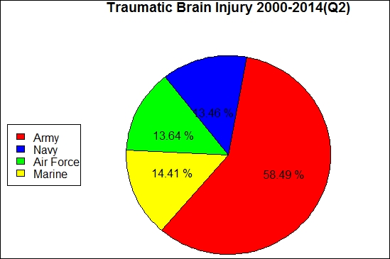
excel - How to not display labels in pie chart that are 0% - Stack Overflow Generate a new column with the following formula: =IF (B2=0,"",A2) Then right click on the labels and choose "Format Data Labels". Check "Value From Cells", choosing the column with the formula and percentage of the Label Options. Under Label Options -> Number -> Category, choose "Custom". Under Format Code, enter the following: How to show percentage in pie chart in Excel? - ExtendOffice Please do as follows to create a pie chart and show percentage in the pie slices. 1. Select the data you will create a pie chart based on, click Insert > I nsert Pie or Doughnut Chart > Pie. See screenshot: 2. Then a pie chart is created. Right click the pie chart and select Add Data Labels from the context menu. 3.

microsoft excel 2016 - How do I move the legend position in a pie chart ... To achieve that, click the Plus button next to the chart and add data labels. Use the options in data label formatting dialog to select what the label should show. And, just as a reminder: if your pie has more than three slices, you're using the wrong chart type. Use a horizontal bar chart instead. Share Improve this answer

Excel pie chart labels inside

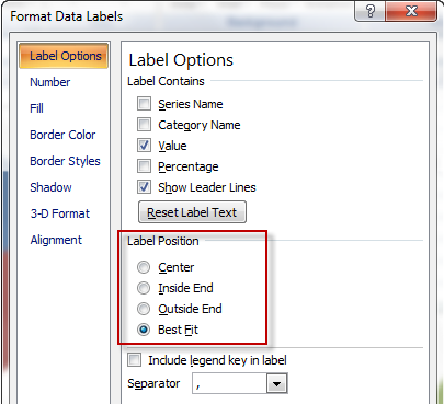
Pie in a Pie Chart - Excel Master Constructing the PIP Chart Drawing a pip chart is the same as drawing almost any other chart: select the data, click Insert, click Charts and then choose the chart style you want. In this case, the chart we want is this one … That is, choose the middle of the three pies shown under the heading 2-D Pie. That's it! That's all you do. Put labels inside pie chart - MrExcel Message Board Click here to reveal answer M Mark W. MrExcel MVP Joined Feb 10, 2002 Messages 11,654 Dec 2, 2003 #2 Select and Format the data labels using the Label Position setting on the Alignment tab. N nicostick New Member Joined Aug 1, 2003 Messages 25 Dec 2, 2003 #3 Perfect! Thanks very much. You must log in or register to reply here. Inserting Data Label in the Color Legend of a pie chart Inserting Data Label in the Color Legend of a pie chart. Hi, I am trying to insert data labels (percentages) as part of the side colored legend, rather than on the pie chart itself, as displayed on the image below. Does Excel offer that option and if so, how can i go about it?

Excel pie chart labels inside. Pie Chart in Excel - Inserting, Formatting, Filters, Data Labels Right click on the Data Labels on the chart. Click on Format Data Labels option. Consequently, this will open up the Format Data Labels pane on the right of the excel worksheet. Mark the Category Name, Percentage and Legend Key. Also mark the labels position at Outside End. This is how the chark looks. Formatting the Chart Background, Chart Styles Excel charts: add title, customize chart axis, legend and data labels ... Click the Chart Elements button, and select the Data Labels option. For example, this is how we can add labels to one of the data series in our Excel chart: For specific chart types, such as pie chart, you can also choose the labels location. For this, click the arrow next to Data Labels, and choose the option you want. excel - Positioning data labels in pie chart - Stack Overflow Sub tester () Dim se As Series Set se = Totalt.ChartObjects ("Inosa gule").Chart.SeriesCollection ("Grøn pil") se.ApplyDataLabels With se.DataLabels .NumberFormat = "0,0 %" With .Format.Fill .ForeColor.RGB = RGB (255, 255, 255) .Transparency = 0.15 End With .Position = xlLabelPositionCenter End With End Sub Multiple data labels (in separate locations on chart) You can do it in a single chart. Create the chart so it has 2 columns of data. At first only the 1 column of data will be displayed. Move that series to the secondary axis. You can now apply different data labels to each series. Attached Files 819208.xlsx‎ (13.8 KB, 264 views) Download Cheers Andy Register To Reply

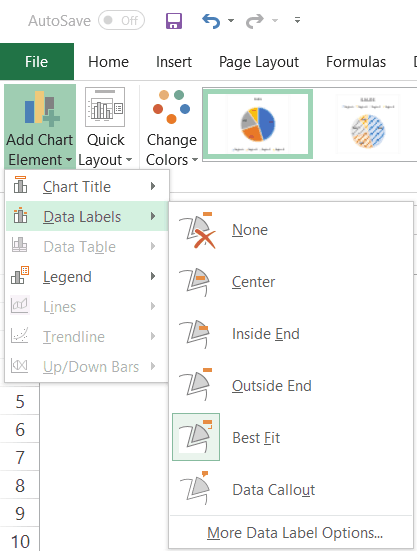
How to Make a 2010 Excel Pie Chart with Labels Both Inside and Outside I am trying to make an excel 2010 pie chart with labels both inside and outside the pie slices. I am following the instructions in this article: How to display leader lines in pie chart in Excel? - ExtendOffice To display leader lines in pie chart, you just need to check an option then drag the labels out. 1. Click at the chart, and right click to select Format Data Labels from context menu. 2. In the popping Format Data Labels dialog/pane, check Show Leader Lines in the Label Options section. See screenshot: 3. How to Make a PIE Chart in Excel (Easy Step-by-Step Guide) Here are the steps to format the data label from the Design tab: Select the chart. This will make the Design tab available in the ribbon. In the Design tab, click on the Add Chart Element (it's in the Chart Layouts group). Hover the cursor on the Data Labels option. How to Create Pie Charts in Excel (In Easy Steps) 6. Create the pie chart (repeat steps 2-3). 7. Click the legend at the bottom and press Delete. 8. Select the pie chart. 9. Click the + button on the right side of the chart and click the check box next to Data Labels. 10. Click the paintbrush icon on the right side of the chart and change the color scheme of the pie chart. Result: 11.

text within a data label in pie chart in excel 2010 doesn't align Re: " Data label text alignment". My memory is hazy, but it may be that some types of pie charts don't provide all options. You may want to see what happens with a different type of pie chart. Also, try padding the text in the data labels with spaces or underscores to get what you want. '---. Office: Display Data Labels in a Pie Chart - Tech-Recipes 1. Launch PowerPoint, and open the document that you want to edit. 2. If you have not inserted a chart yet, go to the Insert tab on the ribbon, and click the Chart option. 3. In the Chart window, choose the Pie chart option from the list on the left. Next, choose the type of pie chart you want on the right side. 4. How to Make a Pie Chart in Excel & Add Rich Data Labels to The Chart! Creating and formatting the Pie Chart 1) Select the data. 2) Go to Insert> Charts> click on the drop-down arrow next to Pie Chart and under 2-D Pie, select the Pie Chart, shown below. 3) Chang the chart title to Breakdown of Errors Made During the Match, by clicking on it and typing the new title. Excel 2010 pie chart data labels in case of "Best Fit" Based on my tested in Excel 2010, the data labels in the "Inside" or "Outside" is based on the data source. If the gap between the data is big, the data labels and leader lines is "outside" the chart. And if the gap between the data is small, the data labels and leader lines is "inside" the chart. Regards, George Zhao TechNet Community Support

How-to Make a WSJ Excel Pie Chart with Labels Both Inside and Outside - Excel Dashboard Templates

I cannot change the default label positions on a pie chart. The option ... Under Add chart element/Data labels, I can only choose "none", "show" or "callout". When I go to "More data label ... Pie charts should have several options: Center, Inside End, Outside End, and Best Fit. ... I've searched extensively for an answer to this problem and the only response seems to be that excel doesn't offer this option for all ...

35 How To Label A Pie Chart - Label Design Ideas 2020

Add or remove data labels in a chart - support.microsoft.com Click the data series or chart. To label one data point, after clicking the series, click that data point. In the upper right corner, next to the chart, click Add Chart Element > Data Labels. To change the location, click the arrow, and choose an option. If you want to show your data label inside a text bubble shape, click Data Callout.

How to Make a PIE Chart in Excel (Easy Step-by-Step Guide)

Edit titles or data labels in a chart - support.microsoft.com The first click selects the data labels for the whole data series, and the second click selects the individual data label. Right-click the data label, and then click Format Data Label or Format Data Labels. Click Label Options if it's not selected, and then select the Reset Label Text check box. Top of Page

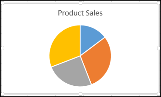
Pie Chart without Labels - Automate Excel

How to Create and Format a Pie Chart in Excel - Lifewire To add data labels to a pie chart: Select the plot area of the pie chart. Right-click the chart. Select Add Data Labels . Select Add Data Labels. In this example, the sales for each cookie is added to the slices of the pie chart. Change Colors

31 Label Pie Chart - Labels For Your Ideas

Pie Chart in Excel | How to Create Pie Chart - EDUCBA Follow the below steps to create your first PIE CHART in Excel. Step 1: Do not select the data; rather, place a cursor outside the data and insert one PIE CHART. Go to the Insert tab and click on a PIE. Popular Course in this category

Share :